
11.1 Quantum number ℓ
Arnold Sommerfeld revised Niels Bohr’s model of the atom (discussed in Chapter 10) in 1915.[1,2] Sommerfeld showed that another number is needed to describe electron orbits besides the shell number (n). This is known as the azimuthal quantum number (ℓ). The azimuthal quantum number describes the orbital angular momentum of an electron, which defines the ‘shape’ of the orbit.
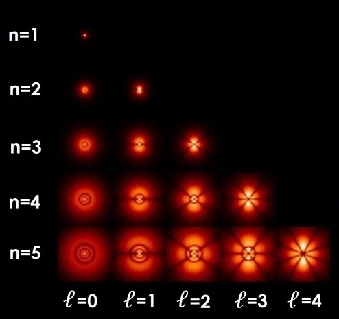
Figure 11.1 |
Hydrogen atom electron orbitals (for magnetic quantum number m = 0). |
Bohr had assumed that orbits would be circular, but Sommerfeld showed that they could take as many shapes as the shell number, i.e. the two electrons in the first shell of helium both have the same shape because the shell number is 1, but the two electrons in the second shell of beryllium can each have different shapes because the shell number is 2. The shapes become more complex the higher the shell number. The maximum number of electrons that are allowed to have the same shape in each shell can be found using the formula,
| Maximum number of electrons with the same shape = 2(2ℓ+1) | (11.1) |
This means that two electrons can have the ℓ = 0 (also known as the s-orbital) shape, six can have the ℓ = 1 (p-orbital) shape, 10 can have the ℓ = 2 (d-orbital) shape, 14 can have the ℓ = 3 (f-orbital) shape, and so on. Figure 11.1 shows the possible shapes that electron orbits can take in the first five electron shells.
11.2 Quantum number m
In 1920, Sommerfeld realised that another number was needed to describe the orbit of electrons.[3,4] This is because the current model could still not explain the Zeeman effect[5] (discussed in Chapter 7), the splitting of spectral lines in the presence of a magnetic field.
Sommerfeld realised that the same ℓ shape can have different orientations in space defined by the magnetic quantum number (m). The maximum number of different orientations can be found using the formula,
| Maximum number of orientations per shape = 2ℓ+1 | (11.2) |
This means that the ℓ=0 shape has one m value, which is designated 0. The ℓ=1 shape can have up to three different m values, which are designated -1, 0, and 1, the ℓ=2 shape can have up to five different m values, which are designated -2, -1, 0, 1, and 2, and so on. Possible orientations for the first four orbital shapes are shown in Figure 11.2.

Figure 11.2 |
Different orientations of the first four orbital shapes. |
A magnetic field causes electrons of the same energy, which would otherwise produce a single spectral line, to have different energies depending on their orientation with respect to the magnetic field. In the case of a cloud of hydrogen atoms, the transition from the second to the first shell produces three lines as about 1/3 gain energy, 1/3 loose energy, and 1/3 are unaffected by the presence of the magnetic field. This explained the normal Zeeman effect.
Sommerfeld was still unable to explain the anomalous Zeeman effect. This is a term used to describe spectra that split into more than three lines in the presence of a magnetic field,[6,7] and it is more likely to occur in lines made from atoms with an odd number of electrons in their outer shell. This meant that many scientists still did not accept that electrons have orbits that are defined by quantised positions and directions in space. Paul Dirac would later explain the anomalous Zeeman effect using another quantum number, s (discussed in Chapter 12).